Generative Adversarial Networks (GANs) have developed extremely quickly in a few short years. It’s easy to find numerous examples of them generating highly realistic artificial samples of things such as human faces or works of art. While the base version of GANs just converts random noise into data samples, there is perhaps more application in using GANs conditionally, when we can use them to convert data between different domains — for example, turning drawings into realistic landscapes. GAN variants that can invert the generation process and recover latent variables from samples are also achieving impressive results in unsupervised learning.
I don’t want to go too far into the foundations of GANs here, as there are already many excellent posts explaining the underlying concepts at various technical levels. See, for example, here, here and here. What I do want to achieve is to explain GANs in a way that turns the underlying concepts into code as clearly as possible. When I got started with GANs, I was initially confused when trying to turn the core ideas into practical implementations. Conversely, the code samples available online didn’t really come with enough discussion to really understand what was going on. Here, we’ll build a GAN in a way that makes the correspondence of the fundamentals and the code as clear as possible (in my entirely subjective view), and that can be extended to different GAN variants with minimum effort in later parts of this series.
In this post, we’ll implement a simple GAN and train it using the MNIST dataset of handwritten numbers. The whole code can be found in a repository on GitHub, where the code for the later parts will also appear. We’ll write everything in the TensorFlow version of Keras. With the end of active development for Theano and the integration of Keras as the official TensorFlow high-level API, it seems that this is, in practice, the future of Keras. This way, we also won’t have to be shy of building TensorFlow-specific extensions in later parts. Nevertheless, most of the code can be converted into the standalone version of Keras simply by changing the import statements.
The Theory
As you probably know if you took a look at the explanations linked above, GANs work by training two neural networks against each other: a generator is trying to generate realistic samples, while a discriminator is trying to distinguish the generated samples from real ones.
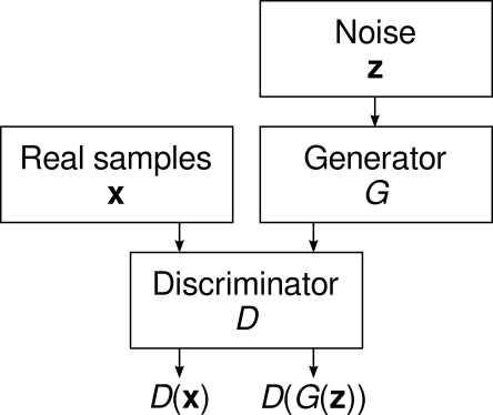
We want to optimize the discriminator to discriminate between real and generated samples as well as possible, while simultaneously optimizing the generator to fool the discriminator as much as possible. Thus, we write the GAN loss functions in terms of the discriminator outputs \( D(\mathbf{x}) \) (for real samples) and \( D(G(\mathbf{z})) \) (for generated samples). The discriminator objective is to minimize the discriminator loss \( L_D \), which is a function that is small when the discriminator is performing well: \[ \min_D E_{\mathbf{x},\mathbf{z}} [ L_D(D(\mathbf{x}),D(G(\mathbf{z}))) ] \] that is, we’re trying to optimize the parameters of \( D \) to minimize \( L_D \). Meanwhile, the generator is trained to minimize its own loss \( L_G \): \[ \min_G E_\mathbf{z} [ L_G(D(G(\mathbf{z}))) ] . \] Clearly, \( L_G \) should be a function that is small when the discriminator is doing poorly. Since the optimization goals are contradictory, in practice we take turns optimizing the discriminator for a constant generator, and vice versa:
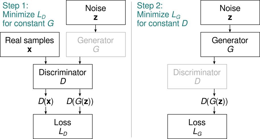
Note how the left branch is not needed for optimizing the generator as \( L_G \) does not depend on the real samples.
For the classic formulation of GANs, the discriminator output is interpreted as the probability that the input image is generated (fake) rather than real (we might as well choose it to be the probability of a real image, but we’ll use this definition here). We then write the discriminator loss as the cross entropy between the correct and estimated answers. As the correct answer is 0 for real samples and 1 for generated samples, we get \[ L_D = -\big ( \log(D(G(\mathbf{z}))) + \log(1-D(\mathbf{x})) \big ) . \] Meanwhile, we want the generator to produce images that the discriminator thinks are real — that is, we optimize using a correct answer of 0. Using cross entropy on the discriminator output again, we get \[ L_G = -\log(1-D(G(\mathbf{z}))) . \]
The Code
How do we turn these concepts into code? First, let’s define our networks. The discriminator is a simple convolutional net with a sigmoid output in the final layer to produce an output between 0 and 1:
def dcgan_disc(img_shape=(32,32,1)):
    def conv_block(channels, strides=2):
        def block(x):
            x = Conv2D(channels, kernel_size=3, strides=strides,
                padding="same")(x)
            x = LeakyReLU(0.2)(x)
            return x
        return block

    image_in = Input(shape=img_shape, name="sample_in")

    x = conv_block(64, strides=1)(image_in)
    x = conv_block(128)(x)
    x = conv_block(256)(x)
    x = Flatten()(x)
    disc_out = Dense(1, activation="sigmoid")(x)

    model = Model(inputs=image_in, outputs=disc_out)

    return model
The generator works in the opposite direction, combining UpSampling2D and Conv2D operations to go from a noise vector to an image, with a tanh output to keep it between -1 and 1:
def dcgan_gen(img_shape=(32,32,1), noise_dim=64):

    def up_block(channels):
        def block(x):
            x = UpSampling2D()(x)
            x = Conv2D(channels, kernel_size=3, padding="same")(x)
            x = BatchNormalization(momentum=0.8)(x)
            x = LeakyReLU(0.2)(x)
            return x
        return block

    noise_in = Input(shape=(noise_dim,), name="noise_in")
    initial_shape = (img_shape[0]//4, img_shape[1]//4, 256)

    x = Dense(np.prod(initial_shape))(noise_in)
    x = LeakyReLU(0.2)(x)
    x = Reshape(initial_shape)(x)
    x = up_block(128)(x)
    x = up_block(64)(x)
    img_out = Conv2D(img_shape[-1], kernel_size=3, padding="same",
        activation="tanh")(x)

    return Model(inputs=noise_in, outputs=img_out)
We try to decouple the generator and discriminator networks from the GAN training machinery. This gives us the maximum flexibility to change the networks without touching the GAN training algorithms, or vice versa. We encapsulate the GAN training into a Python class:
class GAN(object):
    def __init__(self, gen, disc, lr_gen=0.0001, lr_disc=0.0001):
        # Copy attributes...
The lr_gen and lr_disc attributes set the learning rates for the generator and discriminator, respectively. In this example, we’ll leave them at the defaults.
The GAN class has two member functions that we call from the outside: GAN.build and GAN.fit_generator. The build function defines and compiles two GAN training networks, gen_trainer and disc_trainer. First, we create the optimizers (Adam seems to be the usual optimizer of choice for GANs):
    def build(self):
        # ...
        self.opt_disc = Adam(self.lr_disc, beta_1=0.5, beta_2=0.9)
        self.opt_gen = Adam(self.lr_gen, beta_1=0.5, beta_2=0.9)
Then we define the discriminator training network that draws samples from the generator, which is held untrainable:
        with Nontrainable(self.gen):
            real_image = Input(shape=img_shape)
            noise = [Input(shape=s) for s in noise_shapes]

            disc_real = self.disc(real_image)
            generated_image = self.gen(noise)
            disc_fake = self.disc(generated_image)

            self.disc_trainer = Model(
                inputs=[real_image, noise],
                outputs=[disc_real, disc_fake]
            )
            self.disc_trainer.compile(optimizer=self.opt_disc,
                loss=["binary_crossentropy", "binary_crossentropy"])
Note how the code flow is very compact and uses the Keras functional API to follow “Step 1” in the figure above. We break down the loss into two components, the loss for the real images and that for the generated (fake) ones.
The Nontrainable context is defined in the meta module. It simply sets the trainable property in its argument to False. I find this to be a conceptually clear way to do this in Keras; it also removes the need to set trainable = True again manually, and even returns the network in its old state if the code is interrupted by an exception. When I’m working with models interactively, I often like to stop the training manually with Ctrl-C. The Nontrainable context ensures that the models return to their default states when I do that.
The generator training network is built similarly, following “Step 2” in the figure:
        with Nontrainable(self.disc):
            noise = [Input(shape=s) for s in noise_shapes]

            generated_image = self.gen(noise)
            disc_fake = self.disc(generated_image)

            self.gen_trainer = Model(
                inputs=noise,
                outputs=disc_fake
            )
            self.gen_trainer.compile(optimizer=self.opt_gen,
                loss="binary_crossentropy")
Once the GAN is built, we can train it with the fit_generator function, similar to the function of the same name in the Keras Model class. Here’s a decluttered version of the full implementation found in the gan module:
    def fit_generator(self, batch_gen, noise_gen, steps_per_epoch=1, num_epochs=1,
        training_ratio=1):
        # ...
        for epoch in range(num_epochs):
            for step in range(steps_per_epoch):

                # Train discriminator
                with Nontrainable(self.gen):
                    for repeat in range(training_ratio):
                        image_batch = next(batch_gen)
                        noise_batch = next(noise_gen)
                        disc_loss = self.disc_trainer.train_on_batch(
                            [image_batch]+noise_batch,
                            [real_target, fake_target]
                        )

                # Train generator
                with Nontrainable(self.disc):
                    noise_batch = next(noise_gen)
                    gen_loss = self.gen_trainer.train_on_batch(
                        noise_batch, real_target)
Here, real_target is a vector of zeros and fake_target is a vector of ones. We expect batch_gen and noise_gen to be Python iterables, from which we can draw new samples with the next builtin function. batch_gen generates batches of real samples, while noise_gen generates batches of Gaussian noise of the appropriate shape.
We call build and fit_generator from the train module. If you pull the code from the repository, you can run the training code on the MNIST dataset by going to the gan directory and running
python train.py
or you can call the train_gan function manually from an interactive shell. A training that produces decent results should be runnable even on a CPU in a reasonable amount of time, but will probably be much faster on a GPU. You’ll need NumPy, TensorFlow and Matplotlib to run it. It should output a figure called gan_samples.png in the figures directory, which should look like something like this:
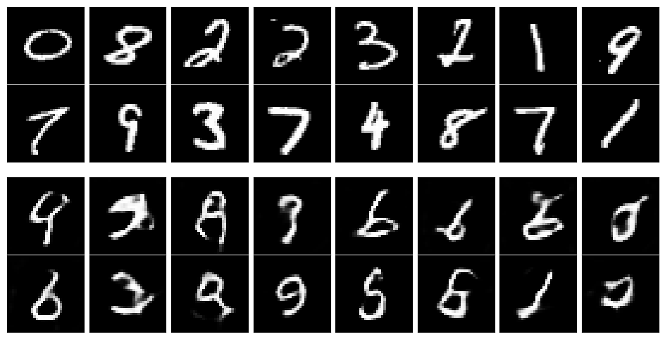 This is hardly perfect but the outputs have a nice resemblance to the real digits. Play around with the amount of training to see how the output changes. And feel free to adapt the code to your own applications! In later parts we’ll explore GAN variants and some more advanced training techniques.