Training GANs remains a bit of an art and one can easily find that small changes in architecture and training procedures make a huge difference to the end results. The effects of various tricks and techniques are not always predictable, but that’s not to say that you can’t save yourself some trouble by adopting some best practices. In my work with GANs, perhaps the one thing that improved my quality of life most was adopting the Wasserstein loss together with the gradient penalty. Despite being introduced only a couple of years ago, Wasserstein GANs (WGANs) have become one of the standard ways to implement GANs.
The Theory
Let’s take a brief look at the theoretical motivation behind the WGAN. If you’re interested in more details, you can find a nice writeup here, or you can of course take a look at the original paper.
In the last part, we looked at the standard GAN loss where the discriminator outputs a probability that its input is fake (generated), and formulated the loss as the cross-entropy between the output and the right answer (0 for real inputs and 1 for fakes). The ultimate goal is to approximate the real data distribution \( P_r \) with the generated distribution \( P_g \), and using the cross-entropy loss corresponds to optimizing the Jensen-Shannon (JS) divergence between the two distributions. The smaller the JS divergence, the closer the two probability distributions are to each other.
The JS divergence is conceptually quite clear, but it has its problems — for instance, its gradient vanishes quickly for two very dissimilar distributions and goes to zero for distributions that have no overlap at all. Fortunately, it’s by no means the only way to measure the distance between two probability distributions. The WGAN formulates the GAN loss based on the Wasserstein-1 or “earth mover’s” distance, defined as the shortest average distance required to move the probability mass from one distribution to another. This quite clearly has a gradient even for completely non-overlapping distributions: as the distributions get further from each other, the Wasserstein distance increases smoothly. The definition of this distance is rather complex, but because of a convenient dual we can write the distance as \[ W(P_r,P_g) = \frac{1}{K} \sup_{\lVert f \rVert_L < K} E_\mathbf{x} [f(\mathbf{x})] - E_\mathbf{z} [f(G(\mathbf{z}))] \] where the supremum is taken over functions that are \( K \)-Lipschitz continuous, which means, very roughly speaking, that the norm of their gradient is nowhere larger than \( K \).
The original WGAN paper constrained \( f \) by clipping the discriminator weights to given range. A better solution was soon invented: instead of hard clipping, we can penalize the gradient to impose a soft constraint on its length. This gradient penalty can be written as \[ (\lVert \nabla_{\hat{\mathbf{x}}} D(\hat{\mathbf{x}}) \rVert - 1)^2 \] where we take the gradient at \( \hat{\mathbf{x}} \), a randomly weighted average between a real and generated sample: \[ \hat{\mathbf{x}} = \epsilon \mathbf{x} + (1-\epsilon)G(\mathbf{z}) \] with \( \epsilon \) selected randomly between 0 and 1.
We find the optimal discriminator by minimizing the Wasserstein distance while constraining the gradients using the penalty term. The discriminator loss is then \[ L_D = D(\mathbf{x}) - D(G(\mathbf{z})) + \gamma (\lVert \nabla_{\hat{\mathbf{x}}} D(\hat{\mathbf{x}}) \rVert - 1)^2 \] and, as in the last part, we optimize for the expectation of this. Written like this, the loss is intuitively quite simple: The discriminator is trained to output values as small as possible for real samples, and as large as possible for fake samples, while the gradient penalty term keeps the weights from blowing up. A loss that has no strict lower bound might seem strange, but in practice the competition between the generator and the discriminator keeps the terms roughly equal. The generator loss is simply to fool the discriminator: \[ L_G = D(G(\mathbf{z})) \] This GAN setup is commonly called improved WGAN or WGAN-GP.
The Code
We use the basic GAN code from last time as the basis for the WGAN-GP implementation, and reuse the same discriminator and generator networks, so I won’t repeat them here. The only change we need to make, since our discriminator output is no longer constrained between 0 and 1, is to change the activation function of the final layer from sigmoid to linear:
def dcgan_disc(img_shape=(32,32,1)):
    # ...
    disc_out = Dense(1, activation="linear")(x)
    # ...
Defining the WGAN loss takes a bit more work. We’ll use the same basic structure in the GAN class:
class WGANGP(object):
    def __init__(self, gen, disc, lr_gen=0.0001, lr_disc=0.0001):
    # ...
We change the GAN loss function to the Wasserstein loss and add the gradient penalty to the outputs of the discriminator (using \( \gamma=10 \)):
        with Nontrainable(self.gen):
            real_image = Input(shape=img_shape)
            noise = [Input(shape=s) for s in noise_shapes]

            disc_real = self.disc(real_image)
            generated_image = self.gen(noise)
            disc_fake = self.disc(generated_image)

            avg_image = RandomWeightedAverage()(
                [real_image, generated_image]
            )
            disc_avg = self.disc(avg_image)
            gp = GradientPenalty()([disc_avg, avg_image])

            self.disc_trainer = Model(
                inputs=[real_image, noise],
                outputs=[disc_real, disc_fake, gp]
            )
            self.disc_trainer.compile(
                optimizer=self.opt_disc,
                loss=[wasserstein_loss, wasserstein_loss, "mse"],
                loss_weights=[1.0, 1.0, 10.0]
            )
The generator training network is just changed to use the Wasserstein loss:
        with Nontrainable(self.disc):
            # ...
            self.gen_trainer.compile(optimizer=self.opt_gen,
                loss=wasserstein_loss)
There are three components here that are not part of the standard Keras toolkit: RandomWeightedAverage to compute the randomly weighted average between real and generated images, GradientPenalty to get the gradient penalty term, and wasserstein_loss to define the loss.
The custom loss is the easiest of the three, albeit a bit of a hack. For the correct answer y_true we pass either +1 (for real images) or -1 (for generated ones) and then multiply the prediction with that value. We just need the mean function from the backend:
from tensorflow.keras import backend as K

def wasserstein_loss(y_true, y_pred):
    return K.mean(y_true * y_pred, axis=-1)
The gradient penalty is a bit more work but still quite simple using a custom layer (subclassed from Layer). We use gradients to compute the gradient and some math with the backend functions to compute the length, then subtract 1 (we leave the squaring to the mean square error loss).
from tensorflow.keras.layers import Layer

class GradientPenalty(Layer):
    def call(self, inputs):
        (target, wrt) = inputs
        grad = K.gradients(target, wrt)[0]
        return K.sqrt(K.sum(K.batch_flatten(K.square(grad)),
            axis=1, keepdims=True))-1

    def compute_output_shape(self, input_shapes):
        return (input_shapes[1][0], 1)
Finally, we need the randomly weighted average. This is similar to the existing Keras merge layers like Add, Subtract and Average so we can use the common framework that those layers use. We get the weights (\( \epsilon \) above) using random_uniform and then compute the average. Everything else below is to manage the shapes:
from tensorflow.python.keras.layers.merge import _Merge

class RandomWeightedAverage(_Merge):
    def _merge_function(self, inputs):
        (x,y) = inputs
        shape = K.shape(x)
        weights = K.random_uniform(shape[:1],0,1)
        for i in range(len(K.int_shape(x))-1):
            weights = K.expand_dims(weights,-1)
        return x*weights + y*(1-weights)
Now we just need to define our targets to fit the WGAN-GP objectives and we’ll be ready to train the GAN:
    def fit_generator(self, batch_gen, noise_gen, steps_per_epoch=1,
        num_epochs=1, training_ratio=1):

        disc_out_shape = (batch_gen.batch_size, self.disc.output_shape[1])
        real_target = np.ones(disc_out_shape, dtype=np.float32)
        fake_target = -real_target
        gp_target = np.zeros_like(real_target)

        for epoch in range(num_epochs):
            for step in range(steps_per_epoch):

                # Train discriminator
                with Nontrainable(self.gen):
                    for repeat in range(training_ratio):
                        image_batch = next(batch_gen)
                        noise_batch = next(noise_gen)
                        disc_loss = self.disc_trainer.train_on_batch(
                            [image_batch]+noise_batch,
                            [real_target, fake_target, gp_target]
                        )
        # ...
Results
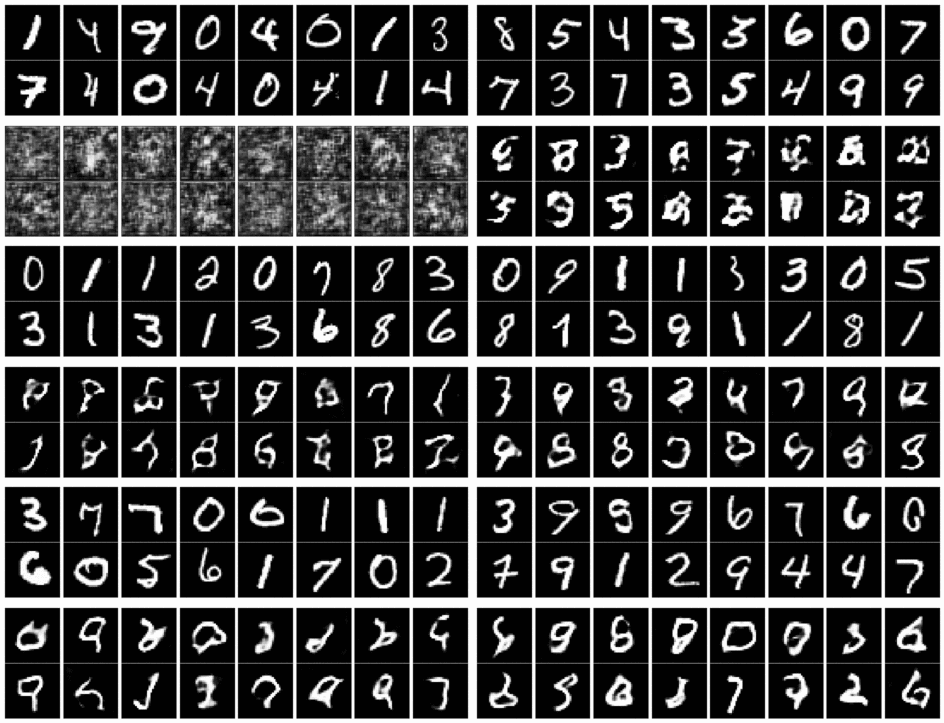
I trained both the traditional GAN and the WGAN-GP on the MNIST dataset, otherwise using the same settings. Here is an animation of the WGAN-GP converging (real images on top, generated on the bottom):

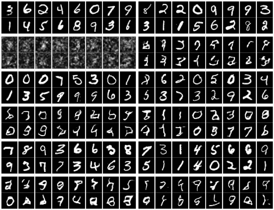
And this is the same with the regular GAN:

Not a huge difference in convergence here, and in both cases we see some systematic biases on each generation (e.g. some digits seem to be overrepresented and the line thickness tends to remain similar in a given batch). Maybe I’m not training long enough, or perhaps the network is not capable enough for the dataset (the dataset is very simple but so is the network). With harder problems, I’ve seen much bigger stability advantages with the WGAN-GP.